FishMet: A simulation model of fish feeding and appetite

Abstract

The FishMet model is a mechanistic, nonparametric, process-based simulation model of fish appetite and feed intake aimed to aquaculture and behavioural ecology. By incorporating mechanistic representation of various processes and signals that control fish appetite, decision-making, behavior and feeding, FishMet can potentially account for complexity, stochasticity, emergent effects etc. The model works at the fine-grained level of individual feed items and individual decisions of the fish. This potentially allow for complex simulations with variable feed, schedules, changing and stochastic environment. In turn, this will use it for decision support in aquaculture.

This documentation applies to the model source code revision r14257.

The document is generated with the AsciiDoc markup processor.

Colophon

The FishMet model development is supported by the iFishIENCi project and The University of Bergen.

1. Introduction

Food intake is necessary to acquire and supply all the energy and required essential nutrients to run the metabolic processes involved in subsistence, activity and growth. Fish feed is one of the most important cost factors in aquaculture. In intensive farming the costs of feed amount to 40-60% of total costs and it is thus important to ensure good control of fish feed use. This means to maximize fish growth and to avoid as much as possible waste from uneaten feed and limit excreted and evacuated matter to the surrounding environment. With todays practice in intensive tanks foods are delivered based on feeding tables that calculate the daily amount of feed administered to the fish tank through the use of mathematical models that combine the number of fish, average individual weight, temperature-based daily growth and the food factor.

In floating cages, and particularly for Atlantic salmon where the net volume has increased significantly over the years the feeding process is controlled manually by an operator who uses remote-controlled underwater cameras to subjectively assess the fish’s appetite by observing fish behaviour and the sinking depth of uneaten pellets. The pellets are delivered through feed lines that runs from silos to nets by a flow of tempered air. This type of feeding control method has been developed over the last decade through a combination of experience and new innovations in feeding infrastructure. However, there is no consensus regarding feeding or feeding control strategy in the industry other than that the camera is the main tool for observation. On the other hand, there are a number of strategies, which include differences in feeding intensity, number and time distribution of meal, and most importantly; what the breeder considers as satiated fish, which has a strong influence on the degree of feed waste that is created. A bottleneck in feeding in all systems is thus a lack of knowledge about the fish’s feeding behaviour and physiology.

However, in such open cage systems it is not uncommon to operate with a feed factor between 1.1 and 1.4, which means a food waste of almost 30% compared to what is possible under optimized conditions where voluntary food intake match administration of food. This practice is a very costly and importantly environmentally unfriendly.

This concept for a model is in line with the paradigm shift in aquaculture where there is being developed a capacity for real-time monitoring and interpretation of fish behaviour. The so called "Fish-Talk-To-Me" concept aims to provide continuous data related to biotic and abiotic factors to the controller. This novel approach is based on understanding the whole organism as an adaptive agent, which not just responds to the environmental input, but acts autonomously, making its own decisions that depend on both the environment and its internal state (Budaev et al., 2019). Its adaptive responses, therefore, are shaped not only by the past and current events, but by expectations of the future that reflect the evolutionary past (Jensen et al., 2020). This agentic view of the fish suggests that a simple one-way interaction would never provide optimal control over its behaviour and growth: continuous feedbacks at different levels are indispensable. A useful metaphor for such approach can be to “converse” with the fish, providing the food and other resources in accordance with what the fish physically needs, “likes,” “wants,” and expects (Castro & Berridge, 2014; Kristiansen et al., 2020). The concept of individual- and group-based fish feedback technology (sensors, communication) aims to provide real-time understanding on the fish´s movement, physiological state, welfare and health.

Agent-based process simulation modelling is an approach where a complex physiological or behavioural process of an individual (modelled as an autonomous agent) is segmented into a sequence of multiple but simple unit submodels based on known equations. These submodels then are combined via an integral flow control that represents the functioning and behaviour of the whole organism. The "flow" then includes various biological entities, such as food mass, energy, information etc.

The integral simulation model, also called a digital twin for feeding will incorporate biological and environmental information to improve predictions of biological response to situations and optimise feeding with measurable outcomes and predictive capacity. Iterative work between modelling and experimental trials, will also aid to train AI algorithms that can be used in automated feeding systems. The AI system will interact—converse—with the fish, based on the digital twin model, to understand its requirements with the aim to optimize the growth and FCR.

Multilevel process-based simulation models based on complex software systems require the ability to accommodate experimental data and to perform model verification, sensitivity analysis and proper validation (Oberkampf & Roy, 2010; Ghasem, 2019). There need to be a formal approach to model and predict voluntary intake, including to state the limits within which the model is designed to operate. Furthermore, a complex digital twin simulation working in concert with a black-box model-free AI system should also adequately respond to unexpected events (Birta & Arbez, 2013). Process-based computer simulation is necessarily based on a robust, testable theory that is implemented in the computer code. There is thus a need in a general account for how intake and diet selection are controlled proximately. Then, experiments should be designed to test specific hypotheses, rather than just to collect more data (Hilborn & Mangel, 1997).

2. Description of the model

2.1. General outline of the model

FishMet, represents a mechanistic, process-based simulation model rather than an analytic model based on few equations. Therefore, it can potentially account for complexity, stochasticity, emergent effects etc. The computational part of the FishMet system is rather complex and follows the principles of process simulations and agent-based modelling1 systems (Railsback & Grimm, 2019). It has been engineered from the start to provide extensibility, interoperability and a plugin-like application within a larger digital twin system. FishMet is a discrete time model running over numerous time steps with the resolution of 1 s. The model works at the fine-grained level of individual feed items and individual fish decisions. This will potentially allow for complex simulations with variable feed, complex schedules and stochastic environment.

dox/lo_draw-model-overview.svg

Figure 1. An overview of the model

The FishMet model is based on available published data that combines observations of fish behaviour and research-based knowledge about the feeding biology (appetite control, digestive physiology and growth). The initial version of the model is developed for Atlantic salmon and rainbow trout, and additional data will be collected during experiments in the iFishIENCi project. An important feature of the model is that feed intake is a calculated output of the model together with behaviour related to feeding. The model will include basic physiology, feeding behaviour and allocation of energy including growth, and also key sensory, biological control mechanisms, but simplified to a level of precision that is useful and applicable in aquaculture.

The factors described above are linked together in a simulation model that integrates knowledge of fish physiology and nutrition and describes food intake, stomach filling, and intestinal passage including digestion and absorption processes in fish. The conceptual model includes new knowledge about the orexigenic and anorexigenic factors that affect appetite and also how peripheral factors such as stomach filling, digestion and plasma levels of nutrients affect feed intake. Gastric filling and intestinal passage will be important elements, and a central part of the model focuses on the changes that occur due to variations in feeding amount and frequency as well as environmental factors such as temperature, and oxygen can affect appetite, feeding behaviour and ultimately food intake.

2.2. Variables and parameters of the model

The list of variables and parameters of the model is given below.

Configuration parameters are given in parentheses, e.g. (food_item_mass). For a full list of model configuration parameters see Default parameters of the model.

2.2.1. Model parameters

$t$: Ambient temperature, C (temperature).
$m_{0}$: Fish body mass at the start of the simulation, g (body_mass).
$S$: Fish stomach filling capacity, g (stomach_capacity).
$G$: Fish midgut filling capacity, g (midgut_capacity).
$c_{0}$: Dry mass of the feed item (food_item_mass).
$E_G$: Gross energy content of the feed, MJ/kg (=kJ/g) (feed_gross_energy).
$F$: Food input rate (food_input_rate) during a meal (food_input_rate).
$\Theta$: Feeding schedule, a time-based Boolean vector that identifies is food provided (meal) or not at the
moment (food_provision_pattern).
$u$: Proportion of water uptake, relative to the initial dry food item mass (water_uptake).
$\delta_i$: Ingestion delay: time to complete the water uptake (ingestion_delay).
$a_{s}$: Water uptake in stomach, logistic function parameter (water_uptake_a).
$r_{s}$: Water uptake in stomach, logistic function parameter (water_uptake_r).
$T_n$: Interpolation grid for food transition pattern in stomach: abscissa (transport_pattern_t).
$R_n$: Interpolation grid for food transition pattern in stomach: ordinate (transport_pattern_r).
$T_{S=0}$: Stomach emptying matrix, an interpolation grid matrix that defines how long does it take to process full stomach calacity of the feed ($S$) until no feed remains in the stomach. The values of this matrix depend on the fish body mass (columns of the matrix) and the ambient temperature (rows of the matrix).
$A$: Digestibility: maximum absorption ratio in the mid-gut, relative to the dry mass of food (absorption_ratio).
$\delta_d$: Digestion delay: time to the start of the absorption process in the midgut (digestion_delay).
$r_{max}$: Michaelis-Meneten food absorption parameter in midgut (midgut_michaelis_r_max).
$M_{MM}$: Michaelis-Meneten food absorption parameter in midgut (midgut_michaelis_k).
$SMR_{t}$ and $SMR_{O}$: Interpolation grid setting how SMR depends on the ambient temperature: temperature and SMR $mg \; O_2 \; kg ^{-1} \; h^{-1}$
(smr_oxygen_temp and smr_oxygen_o2).
$M_{max}$: The longest time a food item can stay in the midgut after absorption is complete and before it is
evacuated (midgut_maxdur).
$a_a$ and $r_a$: Logistic appetite parameters describing how the stomach ($\alpha_s$) and midgut ($\alpha_m$) appetite components depend on the relative stomach and midgut filling (appetite_factor_a and appetite_factor_r).
$r_E$ and $b_E$: Logistic appetite parameters describing how the energy appetite component ($\alpha_E$) depends on the energy
budget (appetite_energy_rate and appetite_energy_shift).
$\alpha_{min}$: Protective appetite threshold for stomach: this is the maximum value of the stomach appetite signal when the overall fish appetite level depends only on stomach filling (appetite_threshold_stomach).
$H$: Duration of the simulation, hours (run_model_hours).

2.2.2. Other variables

$c_{max}$: the mass of the food item after water uptake
$c_{i}$: the mass of a food item at time $t_{i}$

2.3. Feed protocol and fish behaviour

Feed protocol: The model flowchart (Figure 1) starts from the food supply to the modelled environment. The food input can follow an arbitrary protocol, for example, two or three short meals, with any patter of food provisioning.

Feed protocol is defined by a Boolean vector $\Theta$ that describes if the food is provided during a specific time interval (True=1) or not provided (False=0). The internal time interval for $\Theta$ is the model time step, i.e. 1 s. Any arbitrary vector can be defined by providing the vector from a file food_provision_file_name (see the Using food provisioning from csv file section for more details).

Decision to eat: The modelled fish agent is able to perceive every feed item and makes decision to eat or to ignore it based on its level of appetite. All ignored food items are lost (sinking). Further versions of the model can add perception error, for example, due to fish attention and environment (e.g. water clarity).

2.4. Processing food items in the stomach

The period a food item is processed in the stomach can be divided into two unequal parts: (a) water uptake and (b) subsequent transfer to midgut (see Figure 1).

The mass of each food item in the stomach $c_{i}$ depends on the time $t_{i}$ and is calculated as follows.

First, if the time the food item spend in the stomach is smaller than the ingestion delay $\delta_i$, its mass increases through water uptake up to the maximum $c_{max}$ following the logistic equation:

\[c_{i}=c_{0}+\frac{c_{max}-c_{0}}{1+a \times e^{-r \times t_{i}}}\]

Here $a$ and $r$ are the logistic parameters defined by water_uptake_a and water_uptake_r (see List of variables and parameters).

Second, if the time the food item spent in stomach $t_{i}$ is longer than the ingestion delay $\delta_i$ (i.e. after water uptake), its mass decreases from the largest $c_{max}$ value:

\[c_{i}=c_{max} \times I(T_n,R_n,t_{i}-\delta_i)\]

where $I(T_n,R_n,t)$ defines the proportion of $c_{max}$ remaining in the stomach at the time $t_{i}-\delta_i$ that is defined by a cubic spline interpolation (Phillips, 2000) function with the grid values: abscissa $T_n$; ordinate $R_n$. They are defined by the transport_pattern_t and transport_pattern_r parameters.

The interpolant $I$ is normally a monotonously and nearly asymptotically decreasing function of time. Because the pattern is non-parametric, defined by a data-driven interpolation function rather than a specific mathematical equation, any pattern can be easily implemented in the model (e.g. $\frac{dc}{dt}=k c$, see Example below).

Stomach transport: Thus, the resulting overall pattern of food mass changes in the stomach has this form:

dox/plot_stomach_pattern.svg

Figure 2. Stomach transport pattern, this parameter plot can be produced in the model with plot stomach_transport command

Example 1. Example: Calculation of stomach transport pattern grid

Let us water uptake is defined by the standard decay equation:

\[\frac{dc}{dt}=k c\]

The solution to this differential equation is

\[c = c_0 \times e^{k t}\]

Then with $c_{0} = 1.0$ and $k = -0.0001$ one can easily calculate the interpolation grid:

t	c
0	1.000000
5000	0.606530
10000	0.367879
25000	0.082084
30000	0.049787

These values translate to the following configuration options:

transport_pattern_t = [ 0, 5000, 10000, 25000, 30000 ]
# 1.0 * exp(-0.00010 * 5000)
transport_pattern_r = [ 1.000000,  0.606530, 0.367879, 0.082084, 0.049787 ]

2.4.1. Adjustment for temperature and fish mass

Even though the pattern of food transport within the stomach is defined by the $T_n$ and $R_n$ vectors, it depends on the fish body mass and temperature. The dependency is nonparametric and is defined by the stomach emptying matrix $T_{S=0}$ that is based on experimental or published data on stomach emptying (see stomach_emptying_matrix).

An example of the stomach emptying pattern parameter matrix $T_{S=0}$ is given below. Here rows depict the temperature and columns depict the fish body mass.

	50	100	300	500
5	24	35	75	100
10	15	20	50	75
15	9	15	40	50
20	5	10	30	35
22	4	8	29	33

The adjustmednt is conducted in the following way. First, an stomach emptying time $T_{S=0}(t,m)$ is calculated given the specific fish body mass $m$ and ambient temperature $t$ using cubic spline interpolation over the two dimensions (fish body mass and ambient temperature).

Second, an adjustment factor $a_T$ is calculated as

\[ a_T = \frac{T_{S=0}(t,m)}{T{n}^{i}}\]

where $T_{S=0}(t,m)$ is the estimated stomach emptying time for the fish of mass $m$ at temperature $t$ based on the stomach emptying parameter matrix and $T{n}^{i}$ is the last value of the stomach transport pattern array for time that should correspond to zero amount of food in the stomach ($R_{n}^{i} = 0.0$).

Finally, the time (abscissa) vector$T_n$ of the stomach transport pattern is adjusted as $a_T \times T_n$ effectively "stretching" ($a_T > 1$) or "shrinking" ($a_T < 1$) the time dimension to agree with the stomach emptying time given the fish mass and temperature.

The stomach emptying adjustment factor $a_T > 1$ is reported on the stomach transport plot along with the emptying time, temperature and the fish body mass.

Example 2. Example: Displaying the adjusted stomach transport parameter vectors

The adjusted stomach transport pattern that is used in all the calculations can be produced using the
show stomach_transport command in the command line mode:

> show stomach_transport raw
>>> Unadjusted stomach transport
  transport_pattern_t = [0, 1800, 2700, 3420, 4365, 5490, 7200, 9720, 12150,
                         15750, 18450, 20250, 21600, 22950, 24750, 27000]
  transport_pattern_p = [1.00, 0.99, 0.98, 0.96, 0.90, 0.78, 0.61, 0.45, 0.32,
                         0.18, 0.09, 0.05, 0.02, 0.01, 0.01, 0.00]
>
> show stomach_transport adjust
>>> Adjusted stomach transport
    Body mass: 100.00
    Temperature: 16.00
    Stomach emptying time: 14.11 h
  transport_pattern_t = [0, 3385, 5078, 6432, 8210, 10326, 13542, 18282, 22852,
                                29624, 34702, 38088, 40627, 43166, 46552, 50784]
  transport_pattern_p = [1.00, 0.99, 0.98, 0.96, 0.90, 0.78, 0.61, 0.45, 0.32,
                                0.18, 0.09, 0.05, 0.02, 0.01, 0.01, 0.00]
>

2.5. Processing food items in the midgut

First, for each valid food item in the stomach, we calculate the difference between mass of the food item in stomach at the previous time step t-1 and the current step t: $\Delta c_{i}$

\[\Delta c_{i} = c_{i-1} - c_{i}\]

where $c_{i}$ is the mass of the i-th food item in the stomach. This difference is equal to the mass increment that transfers to the midgut.

This increment is set to zero for all food items that stayed in the stomach for less than the $\delta_i$ (ingestion delay, see parameters).

The increment $\Delta c_{i}$ is also set to zero for all food items that have transferred fully from the stomach to the midgut.

Second, the mass of each food item already in the midgut is incremented by the respective increment $\Delta c_{i}$.

\[c_{i} + \Delta c_{i}\]

The age of each food item in the mid-gut is also incremented.

2.5.1. Digestion

There is a delay $\delta_d$ before the food item occurs in the midgut and the absorption process starts. The digestion process is assumed to occur during this period.

2.5.2. Absorption

In the absorption process, certain proportion of the mass of each food item in the mid-gut is subtracted following the equation:

\[c_{i+1} = c_{i} - c_{i} \frac{r_{max} \sum c_{i}}{K_{MM} + \sum c_{i}}\]

where $r_{max}$ and $K_{MM}$ are the Michaelis-Menten equation parameters: the maximum rate and the K constant. Here $\sum c_{i}$ is the total mass of food in the midgut. A plot of this function is Midgut absorption pattern.

dox/plot_midgut_mm_absorp.svg

Figure 3. Michaelis-Meneten absorption function pattern, this parameter plot can be produced in the model with
plot absorption_mm command

Only the food items that stay in the midgut for more than $M_{max}$ are subject to absorption (see digestion).

Note that each food item in the midgut is subjected to Michaelis-Menten absorption depending on the total mass of food in the midgut $\sum V{i}$.

2.6. Evacuation

Finally, each food item that has reached the maximum absorption is checked if it has been processed for more than $M_{max}$ time in the midgut. Those food items are evacuated.

2.7. Energetics of the fish

The energy balance of the fish is conditioned on the absorption calculation at each time step i.

The overall energy balance of the fish is determined by this equation:

\[E_{i} = E_{i-1} + F(\Delta a) - E_{SMR} - E_{AMR}\]

where $E_{i}$ is the energy balance of the fish at time i, $F(\Delta a)$ is the energy that came from increment in the food absorption $a$, $E_{SMR}$ is the energetic equivalent of the standard metabolic rate (SMR) and $E_{AMR}$ is the energetic equivalent of the active metabolic rate (AMR).

2.7.1. Feed energy content

The feed gross energy content is designated as $E_G$ (normally assumed to be 23.0 kJ/g). Then the energy content (kJ) of the feed mass $\Delta a$ (g) can be calculated as

\[F(\Delta a) = E_G \; \Delta a\]

The gross energy of the feed is set as the feed_gross_energy parameter in the model configuration file.

2.7.2. SMR

The standard metabolic rate (SMR) in the rainbow trout is based on the data of Evans (Evans, 1990) Figure 9, and cubic spline interpolation using the following grid (ambient temperature t versus SMR in terms of oxygen uptake):

t ºC	0.0	0.5	5.1	15.2	20.2	25.2	26.2
SMR	38.0	38.0	40.6	67.8	94.6	136.7	145.9

dox/plot_smr_curve.svg

Figure 4. SMR function pattern, this parameter plot can be produced in the model with plot smr_function command

Note that the interpolation grid is set in the model configuration file as smr_oxygen_temp and smr_oxygen_o2 parameters. Therefore, the SMR function can be easily adjusted for other experimental data or species.

Fish oxygen uptake ($mg \; O_2 \; kg ^{-1} \; h^{-1}$ ) is then converted to absolute energy equivalent, kJ for the whole fish with the mass M.

This conversion is based on two equations:

(a) The volume (v, l) of a specific mass (m, g) of oxygen

\[v = m \frac{22.4}{32}\]

(b) energetic equivalent ($E_{SMR}$, kJ) of a specific volume (v, l) of oxygen uptake:

\[E_{SMR} = 19.4 v\]

2.7.3. Activity and locomotion

It is assumed that fish locomotion has two major components: (a) baseline activity $U_{b}$ that depends on the diurnal cycle and (b) additional active locomotion, such as increased activity during feeding.

Baseline activity in the model during the day is defined by the parameter baseline_activity_day and at night, baseline_activity_night.

Appetite-linked activity involves the increased activity $U_{b} \alpha_{a}$ of the fish when its appetite level is non-zero. Here $\alpha_{a}$ is the multiplier factor applied to the baseline activity. The relationship between the fish appetite ($A$) and the factor $\alpha_{a}$ is defined by this equation:

\[\alpha_{a} = k A + b\]

2.7.4. AMR

Active metabolic rate (AMR) is defined by the equation (see (Grottum & Sigholt, 1998)):

\[AMR = 61.6 \times M^{-0.33} \times 1.03^{t} \times 1.79^U\]

where $M$ is the fish mass, $t$ is the ambient temperature and $U$ is the swimming speed.

2.8. Appetite

The level of appetite (A) determines the probability that the modelled fish makes the decision to consume specific feed item. In the current model version, there are three factors determining the fish appetite: (a) stomach fullness, (b) midgut fullness and (c) overall energy balance (improving or worsening). Respectively, there are three appetite components:

stomach appetite component, $\alpha_{s}$,
energy appetite component, $\alpha_{E}$.
midgut appetite component, $\alpha_{m}$,

The stomach and midgut appetite components are calculated based on the logistic equation:

\[1 - \frac{1}{1 + a \cdot e^{-r\cdot m}}\]

where m is the relative stomach (or midgut) filling and a and r are adjustable parameters.

The energy appetite component is defined similarly, using this equation:

\[\frac{1}{1 + e^{-r_E \cdot (- \Delta_E - b_E )}}\]

where $\Delta_E$ is the difference between the two consecutive average energy balance values in units of the SMR, r and b are adjustable parameter (appetite_energy_rate for r and appetite_energy_shift for b).

The overall appetite is determined in such a way that the stomach component exclusively determines it at high stomach fullness (low stomach appetite component $\alpha_{s}$) to to avoid stomach overfilling:

\[A = \left\{\begin{matrix} \alpha_{s}, \alpha_{s} < \alpha_{min} \\ max(\alpha_{s},\alpha_{m},\alpha_{E}) \end{matrix}\right.\]

2.9. Input and output of the model

The model program accepts model parameters as its main input and produces various output plots. Additionally, detailed time-step-wise data can be produced as model output data.

3. Using the FishMet model

The model has two interface modes: command line (CMD) and graphical (GUI). Default parameters of the model and the program are obtained from the configuration file parameters.cfg that should be found in the current directory.

The configuration file in the current directory (or in the location defined by the FFA_MODEL_PARAMETER_FILE environment variable) is mandatory, the model program will not work without it.

3.1. Command line options

FishMet can be controlled with command line options. Both, the Windows style using the slash / and GNU/Linux style prefixed with dash (- or --) are supported. When the program is started with the help switch (-h, --help, /h or /help), it prints a brief help on the terminal. For example:

fishmet.exe /h

The command line switches (options) are listed below:

-h, --help, /h or /help: print brief help
-g, --force-gui, -gui, /gui: force the model to start in the GUI mode.
-run, --run-model, /run: force run model at startup with the default parameters from the configuration file and then exit.
-q, --quiet, /q, /quiet: "quiet mode" with minimum output.
-b, --batch, /b, /batch: "batch mode" with no screen output, useful for running script. Note that GUI is always disabled in the batch mode.

3.2. Environment variables

Some global aspects of the program can also be controlled via the system environment variables.

FFA_MODEL_PARAMETER_FILE: Defines the name of the file that keeps global model parameters. If this environment variable is not set, the default name parameters.cfg is used.
FFA_MODEL_GUI: if set to 1 or yes or true will force the model to start in the GUI mode.
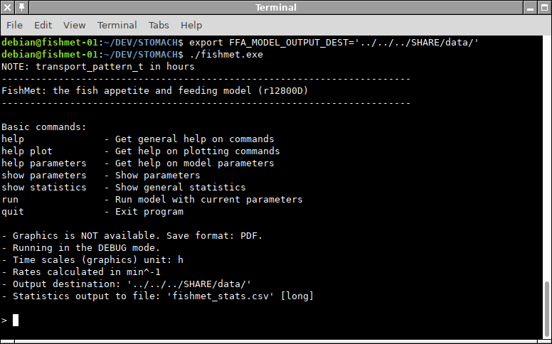
FFA_MODEL_OUTPUT_DEST: sets the output destination as output_dest parameter in the model configuration file. The value set by the environment variable takes priority over the configuration file. Note that the outout destination can also be set using the output_dest parameter in the configuration file, but this environment variable takes priority.
FFA_MODEL_OUTPUT_TAG: sets the model tag that is added to all automatically generated files.
FFA_MODEL_OUTPUT_TAG_CONFIG_REV: causes to determine the model tag that is added to all automatically generated file names from the configuration_version parameter in the main parameter configuration file. See configuration_version parameter.
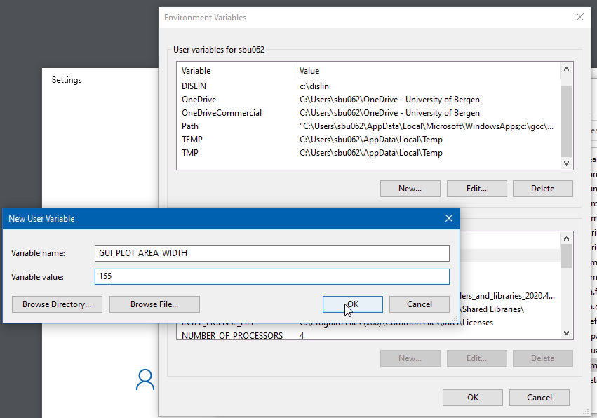
GUI_PLOT_AREA_WIDTH: sets the width of the graphical plotting area. The default value is 110. But if you have a very big computer screen, this may be increased.

The screenshot below provides an example of setting export FFA_MODEL_OUTPUT_DEST on a calculation server.

dox/img_scr_fishmet_envvarserv.png

3.2.1. Windows environment variables

To set environment variable on Microsoft Windows use the set command in the command prompt

set GUI_PLOT_AREA_WIDTH=155

Alternatively, to set a default permanent value that will survive reboots, use Windows Settings dialogue for "Edit environment variables for your account" and add a New environment variable

dox/img_envvar_w10.png

3.2.2. Linux environment variables

Use the shell standard, for example for bash

GUI_PLOT_AREA_WIDTH=155

To make the environment variable permanent, place it into the .bashrc or bash_profile.

3.3. Configuration file

The default configuration parameters of the program (e.g. GUI window) and the model are set in the configuration file named parameters.cfg.

A different model configuration file can be set by setting the environment variable FFA_MODEL_PARAMETER_FILE.

It is a plain ASCII/UTF-8 text file. Each parameter option is set using the option_name = value format. An example configuration file is presented in the Appendix 1.

Array parameters can declared in the same way, with values separated by the white space.

gui_plot_window_page_size = 2970 2100

Also, arrays can use the Python syntax, e.g.

gui_plot_window_page_size = [2970, 2100]

R syntax, e.g.

gui_plot_window_page_size = c(2970, 2100)

This allows reusing the default parameters file in third-party Python or R scripts (e.g. source("parameters.cfg") in R) .

Any line starting from # is considered a comment and is ignored. An example is shown below:

# 2.6. Water uptake pattern over time is defined by the logistic equation
#  c /(1+a*%e**(-r2*t)); where c is the upper limit of the mass,
#  a and r are logistic parameters and %e is natural logarithm base.
# Thus, water uptake dynamics is defined by two additional logistic
# parameters: `water_uptake_a` and `water_uptake_r`
water_uptake_a = 200.0

The parameters and options can be placed in the configuration file in any order.

3.3.1. Program options

interface_graphical

default program interface type, graphical true or command line false.

output_dest

Output destination (usually directory): all plot and output data files will be saved there. The default value is if this variable is absent or directory is not writeable is the current directory. This parameter affects the program behaviour only in the command line user interface and not in the graphical user interface. Note that fish object data save fish_object_data is saved exactly into the fish_object_file because this is non-human readable internal binary data not intended as the model output. The destination can refer to destination directory or output file name prefix. In the former case it should terminate with the operating system specific directory delimiter (e.g. / on GNU/Linux or \ on Microsoft Windows). If the value of output_dest does not terminate this way, it will refer to the file prefix. It is important that the output destination can also be set with the FFA_MODEL_OUTPUT_DEST environment variable, which takes priority over this configuration file parameter. The following outputs are saved to the output_dest:

output plots produced by save command;
output arrays by save model_output;
rate arrays by save rate_output;
output statistics by output stats and append stats.

time_plots_unit_scale

Scale units for the time-based plots 1=sec, 2=min, 3=hours.

rate_unit_scale

Default time unit scale for calculating rates. Rate unit is set as digit: 1=s-1, 2=min-1, 3=h-1.

plot_scale_relative

define whether to use the raw absolute or relative for some of the time-based plots, e.g. stomach and midgut mass dynamics. true means relative scales, i.e. stomach or midgut food mass plot displays filling relative to the total capacity, false means that absolute food mass is used.

rate_interval

default discretization interval in minutes that is used to calculate rate, e.g. this interval is used to plot the ingestion rate

gui_plot_window_page_size

default page size (height, width) for the GUI plot window in pixels.

gui_plot_area_width

default width of the plot output area in pixels.

gui_plot_area_aspect

default aspect ratio (height/width) of the plot output area.

configuration_version

defines the configuration version tag that is added to all automatically generated output files. The tag should be defined using Subversion "$Revision: 1234 $" keyword. It is then parsed to exclude everything except the revision number, adding "conf_r" prefix. (so configuration_version = "$Revision: 1234 $" translates to "conf_r1234". Note that this behaviour is enabled if the environment variable FFA_MODEL_OUTPUT_TAG_CONFIG_REV is set to any value and disabled otherwise.

food_provision_file_name

This variable defines the file name that contains the food provision scheduling. This file should be in CSV format or a single-column plain text. In a multi-column CSV file, the last column is assumed to contain the feed scheduling. Scheduling is encoded by zero and non-zero values by minute (or by second if food_provisioning_file_by_s is set to TRUE). Here any non-zero value means that food is provided during the respective minute interval, zero means that food is not provided. The file is intended to describe the temporal pattern for 24 h, any longer sequence is discarded. All missing values used for filling the remaining minutes to complete the 24 h are zeroes, i.e. food not provided. The pattern is then propagated for all 24 h periods if food_provision_file_repeat is TRUE or applied once if food_provision_file_repeat is FALSE. Note that the file takes priority over the food ononing pattern defined in food_provision_pattern. Example: food_provision_file_name = "../file_name.csv"

food_provision_file_repeat

A logical flag that defines if the feed scheduling pattern defined by the food_provision_file_name file will propagate to all 24 h periods or applied just once to the first such period. The default value is TRUE.
Example: food_provision_file_repeat = TRUE

food_provisioning_file_by_s

Global logical flag that defines if the feed scheduling pattern defined by the food_provision_file_name file represents the data for each time step (s) (if TRUE) or by minute (FALSE). The default value is FALSE i.e. data are given for each minute.
Example: food_provisioning_file_by_s = FALSE

stats_output_file

The name of the CSV file to save general output statistics for specific run of the model.
The default name is "fishmet_stats.csv"
Example: stats_output_file = "data.csv".

stats_output_long

This is a logical parameter that defines if the output stats are saved using the long or short format. In the first case, both the input parameters and the output stats are saved/appended into the CSV file. Note that the default value is TRUE.
Example: stats_output_long = TRUE

stats_output_prediction_stamp

This parameter define if the prediction timestamp is produced in the output stats file. This timestamp then takes the model execution timestamp and adds the time equivalent to the run_model_hours simulation duration. The default value is FALSE. All timestamps are produced in the following format: 2023/07/21 03:09:50.
Example: stats_output_prediction_stamp = TRUE

fish_object_file

The name of the binary file to save the fish object data, i.e. all data for the model fish allowing to resume simulation from a specific fish state (stomach and midgut content, appetite level etc). The default file name is fishmet_fish_state.bin. Note that the file name must have the .bin file extension, otherwise it is not accepted.
Example: fish_object_file = "persistent_data_1.bin"

stomach_emptying_matrix

The name of the CSV data file that defines the stomach emptying parameter matrix, an interpolation grid matrix that defines how long does it take to process full stomach calacity of the feed until no feed remains in the stomach. The matrix defined in this file determines stomach emptying time for a range of fish body mass (columns) and ambient temperatures (rows).

An example of the stomach emptying matrix is provided below:

 ,   50,  100,  300,  500
5,   24,   35,   75,  100
10,  15,   20,   50,   75
15,   9,   15,   40,   50
20,   5,   10,   30,   35
22,   4,    8,   29,   33

Here the rows define ambirnt temperatures (5,10,15,20,22 C) and columns refer to the fish body mass (50, 100, 300, 500 g).

3.3.2. Default parameters of the model

The parameters of the model described below can de defined in the parameter file or set during the runtime using the command line or graphical user interface. They can also be defined in a batch script file.

run_model_hours: Total number of hours for which the simulation is run. It translates into the raw time steps internally as T = H x 3600, where T is the number of time steps, H is the run_model_hours parameter and 3600 is seconds per hour. Example: run_model_hours = 24.
daytime_hours: Default daytime duration, hours. The night time duration is defined as 24-daytime_hours. Note that feeding activity occurs only during the day time and not at night. Example: daytime_hours = 12.
day_starts_hour: Default hour at which the daytime is normally started. It is also the initial offset for day at the start of the simulation. Example: day_starts_hour = 6.
temperature: Ambient temperature ºC. Example: temperature = 14.
body_mass: Fish body mass at the start of the simulation, g. Example: body_mass = 10.0.
body_mass_override: Override body_mass value from fish object file (see fish_object_file) with input parameter value.
baseline_activity_day: Baseline locomotor activity, swimming speed SL/s, during the day as defined by daytime_hours parameter. + Example: baseline_activity_day = 2.5.
baseline_activity_night: Baseline locomotor activity, swimming speed, SL/s, during the day as defined by daytime_hours parameter. + Example: baseline_activity_night = 0.5.
stomach_capacity: fish stomach mass, max. filling capacity, g. Example: stomach_capacity = 5.0.
midgut_capacity: fish midgut mass, max. filling capacity, g. Example: midgut_capacity = 10.0.
stomach_midgut_automatic: logical flag determining, when TRUE, that stomach_capacity and midgut_capacity are continuously automatically recalculated based on the body mass body_mass. Note that this can override any fixed parameter values set by the parameter values stomach_capacity and midgut_capacity.
Example: stomach_midgut_automatic = True
absorption_ratio: Absorption ratio in the midgut, relative to the initial mass of food. Example: absorption_ratio = 0.7.
ingestion_delay: Delay after ingestion, min. Water uptake occurs during the delay. Example: ingestion_delay = 30.
water_uptake: Proportion of water uptake, relative to the initial food item mass. Example: water_uptake = 0.20.
water_uptake_a: Water uptake pattern over time is defined by the logistic equation $\frac{ c }{ 1+a e^{-r^2 t} }$, where c is the upper limit of the mass, a and r are logistic parameters and e is natural logarithm base. The a and r parameters of the equation refer to the water_uptake_a and water_uptake_r parameters. See also water_uptake_r. Example: water_uptake_a = 200.0.
water_uptake_r: Water uptake pattern over time is defined by the logistic equation $\frac{ c }{ 1+a e^{-r^2 t} }$, where c is the upper limit of the mass, a and r are logistic parameters and %e is natural logarithm base. The a and r parameters of the equation refer to the water_uptake_a and water_uptake_r parameters. See also water_uptake_a. Example: water_uptake_r = 0.01.
digestion_delay: Delay of digestion, min. This refers to the time interval from the moment the food item gets into the mid-gut until absorption of the food starts. Example: digestion_delay = 20.
midgut_maxdur: The maximum duration a food item can be processed in the fish midgut, min. If it stays in the mid-gut for any longer time, it is evacuated. Example: midgut_maxdur = 180.
transport_pattern_t: Grid array defining the food transport pattern in the stomach. This array defines the time grid for interpolation. Note that normally it takes several hours until the food item fully disappears from stomach (gastric emptying time). This parameter can be set either in hours (small numbers) or in raw seconds (large numbers) and the correct time unit is normally autodetected by the program. See also transport_pattern_r.
Example (s): transport_pattern_t = 0 3000 15000 21600
Example (hours): transport_pattern_t = 0, 0.8, 4, 6
transport_pattern_r: Grid array defining the food transport pattern in the stomach. This array defines the proportion of food mass left in stomach at each level of transport_pattern_t array. See also transport_pattern_t.
Example: transport_pattern_r = 1.0 0.6 0.01 0.0.
appetite_night: Fish appetite at night. This value is normally low because the fish do not feed at night. If the value is absent or negative, fish appetite does not reduce at night.
Example: appetite_night = 0.1
appetite_factor_a: Appetite factor is defined by the logistic equation: $\frac{ c }{ 1+a e^{-r^2 t} }$. This parameter refers to a. See also appetite_factor_r. Example: appetite_factor_a = 50000.0.
appetite_factor_r: Appetite factor is defined by the logistic equation: $\frac{ c }{ 1+a e^{-r^2 t} }$. This parameter refers to r. See also appetite_factor_a. Example: appetite_factor_r = 20.0.
appetite_threshold_stomach: Protective appetite threshold for stomach: this is the maximum value of the stomach appetite signam when the overall fish appetite level depends only on stomach filling. Setting a sufficiently low value provides a way to protect stomach from overfilling.
Example: appetite_threshold_stomach = 0.2
appetite_energy_rate: Logistic appetite parameter describing defining the energy appetite component dependence on the energy budget.
Example: appetite_energy_rate = 40.0
appetite_energy_shift: Logistic appetite parameter describing defining the energy appetite component dependence on the energy budget.
Example: appetite_energy_shift = 0.2
activity_appetite_factor: Activity appetite factor determining how fish locomotor activity increases with increasing appetite.
Example: activity_appetite_factor = 0.5
midgut_michaelis_r_max: Michaelis-Meneten food absorption parameter in midgut, r_max, relative to the mass of the food item. Rate is per second, the basic discrete step of the model. E.g. 0.8 means that 80% of the food item mass can be absorbed at maximum. See also midgut_michaelis_k. Example: midgut_michaelis_r_max = 0.9.
midgut_michaelis_k: Michaelis-Meneten food absorption parameter in midgut, K_M, relative to the total midgut capacity (e.g. 0.25 means a quarter of the total midgut mass). See also midgut_michaelis_k. Example: midgut_michaelis_k = 0.25.
smr_oxygen_temp: Interpolation X axis grid defining the SMR function on the temperature ºC.
smr_oxygen_o2: Interpolation grid Y axis defining the SMR function on the temperature. SMR unit is $mg \; O_{2} \; kg^{-1} \; h^{-1}$.
food_item_mass: Basic dry mass of one food item (g). Example: food_item_mass = 0.25.
feed_gross_energy: Gross energy content of the feed, MJ/kg (= kJ/g) Example: feed_gross_energy = 23.0.
food_input_rate: Rate of food item input, per min. Example: food_input_rate = 6.0.
food_provision_pattern: Food provision patterning is determined by an array defining the time intervals (min) when food is provisioned and not provisioned e.g. a value of 10 230 means 10 min food is given followed by 230 min not given. Note also that any arbitrary food scheduling can be obtained by encoding periods of food provisioning and not provisioning in the food_provision_file_name parameter. Example: food_provision_pattern = 10 230.
feed_start_offset: The offset (delay, min) to start feeding at the beginning of the 24 hour period. The feeding pattern defined by food provision pattern starts every 24h period after this offset. For example, if the offset is set to 180 min, this means that the first feeding session defined by the food_provision_pattern begins 3h (180 min) after the start of the day. Example: feed_start_offset = 180
stomach_emptying_matrix: The stomach emptying parameter matrix, an interpolation grid matrix that defines how long does it take to process full stomach calacity of the feed until no feed remains in the stomach. The matrix is defined in a file set by stomach_emptying_matrix.

All parameters and formula symbols are listed in the List of variables and parameters.

3.3.3. Examples

Using food provisioning pattern

food_provision_pattern = 10 20

Translates to the following feeding pattern

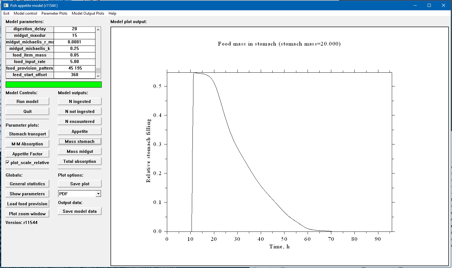
3.4. Graphical user interface

The graphical user interface (GUI) allows interacting with the FishMet model using the familiar point and click mode. The main program window is split into several panels. In the upper left one can find a table of the model parameters that coincide with the configuration file parameters and model parameters in the command line interface. Underneath, one finds buttons for running the model, exiting program and producing various plots as well as saving the output data.

The right panel of the program is devised to show the plots. Note that plots can be saved in several graphical formats. The "WMF" (Windows MetaFile) is recommended on the Microsoft Windows platform because it is a vector graphics that can be scalable and therefore result in high quality. WMF images can be easily inserted in various Microsoft Office documents.

A screenshot of the FishMet GUI is shown below.

dox/img_scr_gui.png

3.4.1. Requesting the GUI mode

To run the program in the GUI mode one can use the -g and similar command line option. Alternatively, it can be requested using an environment variable. Also, one can configure the program to run in the GUI mode by setting the option "interface_graphical = true" in the configuration file. Also, on the Microsoft Windows platform, the program includes the fishmet.vbs VBS script that runs the GUI and suppresses the terminal window.

3.4.2. Saving model data

dox/img_scr_dat2_gui.png

3.5. Command line user interface an scripting

3.5.1. Commands

The command line user interface involves typing commands in the program shell. Alternatively, a set of commands can be provided in a batch script file.

help

Get brief help on the commands. Several subcommands can be used: parameters, plot.

run

Run the model with the default parameters. Alternative alias: start.

reset

Reset all model parameters to the default values from the configuration file. Alternative alias: restart.

quit

exit the program.

set

Set any model parameter defined in Model parameters. Example: set run_model_hours=24. Another use of the set command is to define the output format for saving plots (see save command): set format or set save_format, then define one of the possible output formats: PDF, PNG, SVG, BMP, GIF, EPS, WMF, CGM. This command is also used to define rate interval: set rate_interval as well as to define override flags.

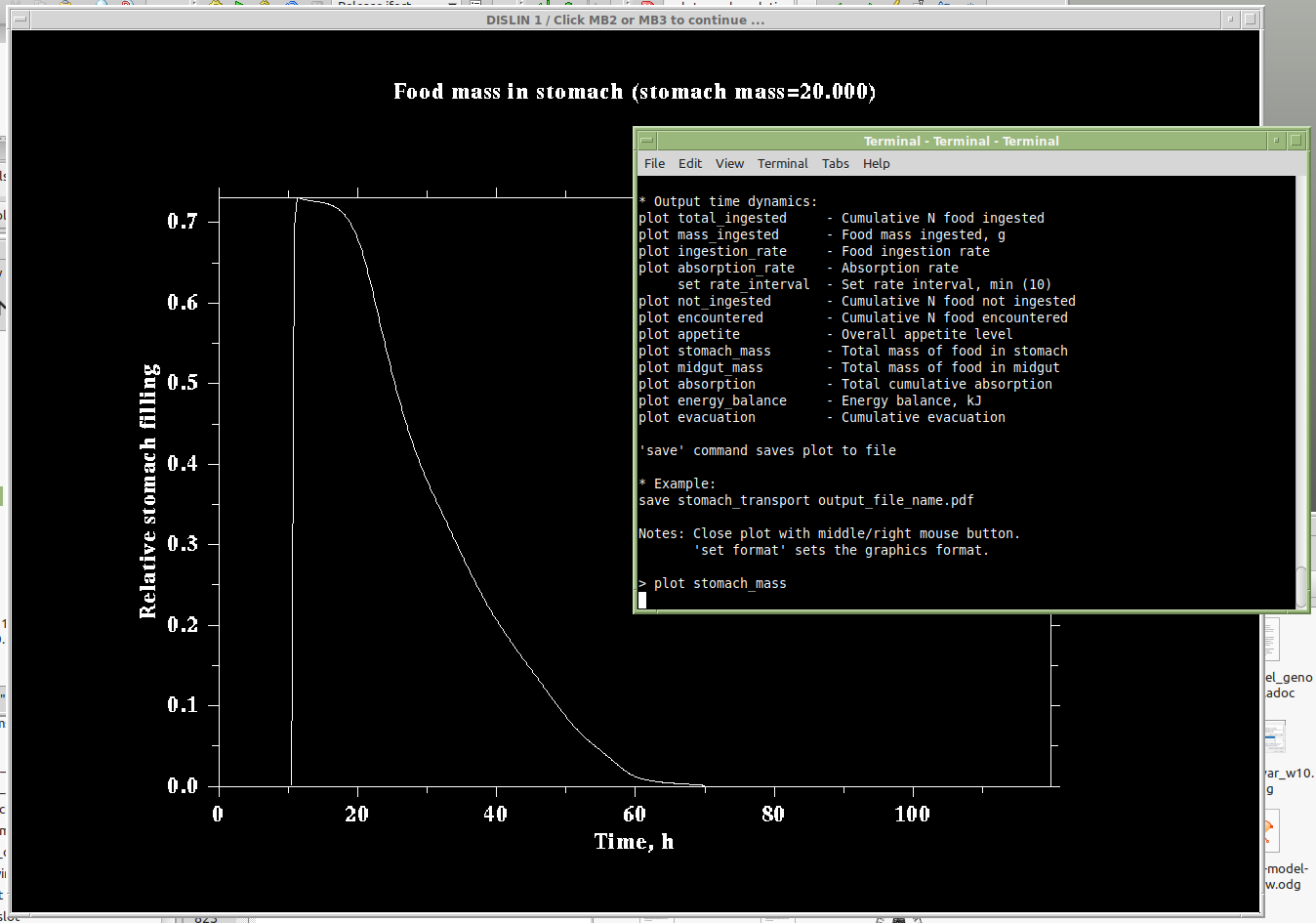
plot

Produce parameter plots or model output plots. To save a plot to a disk file, use the related save command. Rate plots can have different rate interval using set rate_interval command. Example: plot stomach_transport.
Subcommands:

stomach_transport - Stomach transport curve;
absorption_mm - Michaelis-Menten absorption;
appetite_factor - Appetite factor;
smr_function - SMR pattern function;
total_ingested - Cumulative N food ingested;
mass_ingested - Food mass ingested, g;
ingestion_rate - Food ingestion rate;
absorption_rate - Absorption rate;
not_ingested - Cumulative N food not ingested;
encountered - Cumulative N food encountered;
appetite - Overall appetite level;
total_stomach - Total mass of food in stomach;
total_midgut - Total mass of food in midgut;
absorption - Total cumulative absorption;
energy_balance - Energy balance, kJ;
body_mass - Body mass, g;
growth_rate - Growth rate, g/min;
sgr - Specific growth rate, g/min;
activity - Locomotor activity, SL/s;
evacuation - Cumulative evacuation.

save

Save a plot defined as in the plot subcommand. This command also requires two additional parameters: plot type as in plot and the file name. Example: save stomach_transport plot_01.pdf.
Another use of this command is for saving model output data (CSV formatted table):

model_output, output_arrays or output_data - model output arrays;
rate_output, output_rate, rate_data - model rate data (using default rate interval,
see set rate_interval command to change it).
fish_object_data or fish - save full fish object data allowing to resume simulation using the load command. Note that the file name for the fish object is defined by fish_object_file.

load

fish_object_data or fish - load full fish object data allowing to resume simulation. Note that the file name for the fish object is defined by fish_object_file.

show

This command is used to print specific model parameters.

show params or params: print all parameters of the model;
show stomach_transport with optional raw or adjust: show stomach transport unadjusted or adjusted to temperatrure and fish mass;
show stomach_emptying: display the current stomach emptying matrix
as obtained from the stomach_emptying_matrix;
show version: print the program version;
show timesteps: print the total number of timesteps;
show stomach_transport raw, show stomach_transport adjust: display the unadjusted and adjusted stomach transport grid arrays: transport_pattern_t and transport_pattern_r;
show save_format or show format: print the graphic output format (PDF, PNG, SVG, BMP, GIF, EPS, WMF, CGM, CSV).
show plot_scale_relative: print if the time plots show raw data or relative values (e.g. stomach filling relative to the total stomach capacity).
show statistics or show stats: show general model output statistics.

adjust stomach_transport

Adjust the stomach transport parameter arrays for the body_mass and ambient temperature. See also stomach emptying matrix.

output statistics

Initiate output of the general model statistics into stats_output_file csv output data file. Note that this results in writing the column headers and the first row of the data. All subsequent data output should use the append statistics command. Warning: The output command will overwrite any existing CSV file, be careful!.

append statistics

Append general statistics data for the current run of the model. Note that the first output should use the output statistics command.

shell

Execute some operating system specific command. This command can be useful, for example, for checking files from within the model program, moving files, deleting temporary files etc. Example: shell dir /w (this will show all files in the working directory on Windows without size, timestamp and other details).

Override flags:

The load command that loads the fish object data to resume simulation works such that when the simulation is resumed, fish parameters (e.g. body_mass) are obtained from the fish object data (see fish_object_file) rather than the model parameters, either defined in the parameter file or set command. This ensures smooth continuous simulation over many "resumes." However, there is a method to override the fish object data parameters with those explicitly defined by set or parameter file. It is done by setting the body_mass_override flag to TRUE with set command.

Example: "set body_mass_override = True": the value of the body_mass will be obtained from input parameter rather than fish object file.

Screenshot:

An example screenshot of the command line user interface is presented below.

dox/img_scr_cmd.png

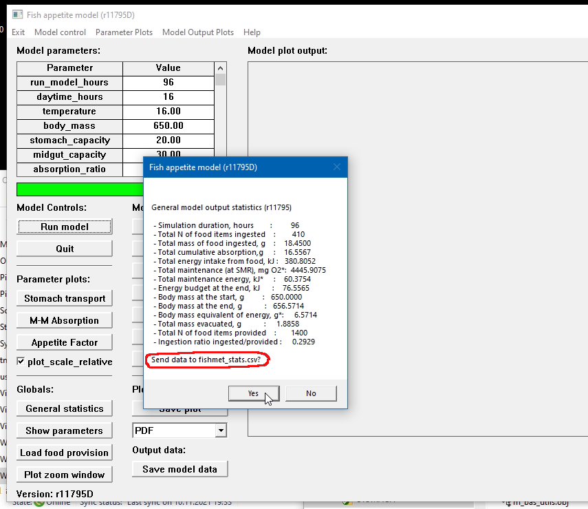
3.5.2. Saving model data

The model can output two kinds of data:

Model output arrays: the data for the time-based dynamics of various variables over time steps of a single model run. To save the model output arrays use the save command: save statistics file_name.csv.
General output statistics: summary statistics of a single model run. To display general output statistics for the current run, use the show command: show statistics. To save these data for the current run, use the output and append commands: output statistics and append statistics. The difference between output and append is that the former saves the header line with variable names as the first line of the output file. The later saves just the data row for the current model run. Thus, when conducting computational experiments with multiple model runs use output statistics after the first run and append statistics after all subsequent runs. Note that to set the file name for these summary data one has to set stats_output_file configuration parameter.

An example of this approach is given below. The model was run (run command) once with default parameters. To inspect the general statistics on screen, the show statistics command was used. Then, output statistics was issued to start saving run by run data to the default CSV output file.

dox/img_scr_dat1_output.png

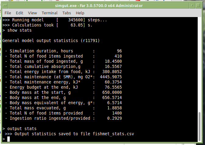
Subsequently, one just needs to issue append statistics command after any additional run of the simulation.

The general output statistics data for each run is simply appended to the same output CSV file on each invocation of the append command. Therefore, there is no limitations on the workflow. For example, on can exit the model program, restart it and keep `append`ing data from additional model runs. Or even start the mode in the GUI mode and append general statistics data to the same file. One possible scenario is to run models in the batch mode on several networked hosts and save data on a shared drive, the only limitation in such a case is that simultaneous writing should be avoided (e.g. by a write-lock file issued by the orchestrating system).

3.5.3. Batch operation

The model can be run repeatedly in the batch mode using a FishMet script file that contains all the commands that should be executed, such as setting model parameters, generating plots, saving data. The run command should also be included for actually running the model.

An example of a FishMet script is shown below:

# FISHMET command script: fishmet_commands.script

# Setting global parameters
set stats_output_file zzz.csv

# Model parameter set, all other parameters are set default
set temperature = 5
set food_input_rate = 5
set body_mass = 50.0
set stomach_capacity = 7.1695
set midgut_capacity = 10.7542

# Run the simulation
run

# Generate outputs

# Plots
save ingested zplot-ingested.pdf
save ingestion_rate zplot-ingest-rate.pdf
save absorption zplot-absorp.pdf

# Statistics
output statistics

Running such a script is done as follows (assuming the command file name is fishmet_commands.script):

fishmet.exe --batch < fishmet_commands.script

The --batch command line option guarantees that the script is running strictly in the command line mode and suppressess all extra output.

A FishMet command script can also be automatically generated. An example command script that generates a combination of parameters is given in Appendix 2.

3.6. FishMet server

The FishMet model system also implements a series of server components that allow execution of the model on a remote server, and data exchange over authenticated http requests. For this, an application programming interface (API) has been developed. This allows to integrate the FishMet model into any cloud-based fish farm management/control system, for example, providing routine predictions of the fish behaviour and growth as well as arbitrary scenario modelling.

3.6.1. iBOSS

The FishMet model has been integrated into the iFishIENCi Biology Online Steering System (iBOSS). iBOSS is aimed to improve production control and management for all fish aquaculture systems. Within iBOSS, smart function can be implemented to take advantage of data from multiple sources to give better insight for the farmer, optimize production, better production planning, etc. The iBOSS Smart Feeding aims at maximizing feed utilization while minimizing environmental impacts, by optimizing the efficiency of the presentation of feed to the fish in relation to fish state, behaviour, environmental conditions and species to maximize growth and reduce feed loss. Multiple AI models are being developed, each adding its own interpretation of the feeding efficiency. All interpretations are integrated in an automated decision-making system to give the feeder signal to either increase or decrease feeding.

3.6.2. Server components

The FishMet server components include: (a) a web server; (b) FishMet software, (c) user or system service that controls all interactions with the model over the network, (d) chatbot-based server and service control interface. The data API is based on the industry-standard JSON format. The output of the model and model predictions are downloaded from the FishMet server in the CSV format.

Data produced and consumed by FishMet: FishMet accepts data on the environment conditions, the feeding protocol, various parameters of the fish morphology and physiology. The output of the model is then the pattern of the fish feeding behaviour (e.g., ingesting food items), its internal state (e.g., the level of appetite) and parameters of the gastrointestinal system functioning (e.g., stomach and gut fullness, absorption, evacuation of faeces). There is also approximations for growth, FCR, and oxygen uptake.

The flow of the interaction: The interactions between the iBOSS and FishMet is presented on the diagram below. Basically, the FishMet model execution is triggered on demand by sending the model parameters to the FishMet server as shown on the interaction diagram. The server components are quite generic and can be adapted for other systems.

All the interactions are initiated on-demand by iBOSS.

Input JSON data file is transferred from iBOSS simulator wrapper to the FishMet server (https PUT request). This triggers generation of the model command script, which will do the following:
- Get the JSON data from iBOSS as input parameters; It will also translate the feed scheduling data to the FishMet format;
- generate FishMet command script the defines the modelling scenario, translates food scheduling data to the FishMet format and is executed by the FishMet executable program;
- run the FishMet executable with the Fishmet command script;
- send notifications about the triggered model execution, along with the FishMet command script that is generated and further notification when FishMet computation is finished.
- archive and backup the input and output data for later reference, testing, debugging etc.
Once the simulation is finished and the FishMet output data are available in the FishMet share folder, available over https, WebDAV or sftp protocols.

More information on the server components are available at https://fishmet.uib.no and https://fishmet.uib.no/doc/srv/server_doc.html.

3.7. Tips and tricks

3.7.1. How to restart next simulation from a previous state

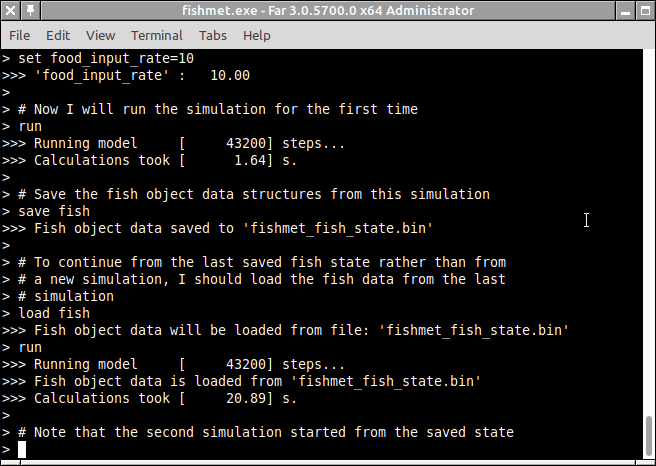
It is possible to save full fish object data at the end of the simulation into a complete data structure and reload it to start the next simulation from exactly this state. For example one may have a simulation of fish for 24 hours starting from an empty stomach. Then, after these 24 hours, there is some food in the fish stomach and midgut and one can restart the next simulation from this state rather than from an empty state.

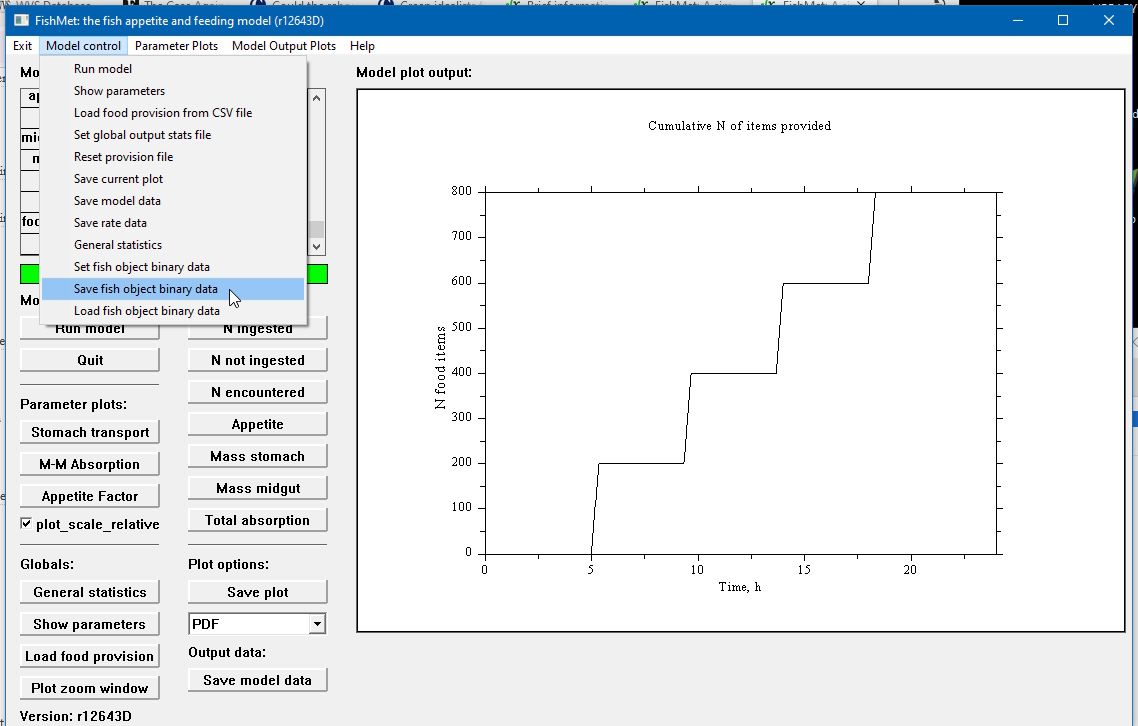
To do this one needs to save the fish object data to a binary file using the "save fish" command in the command line mode or Save fish object data menu item (Model control drop-down menu) in the graphical mode.

The file name is defined by the fish_object_file parameter and can be changed using the set fish_object_file in the command mode. There is also a menu item for this in the graphical mode.

Then, what is necessary is to (a) save the fish state at the end of the simulation and (b) load this file before the next simulation starts. The screenshot below illustrates this in the command line mode.

dox/img_scr_rerun_fish_object.png

And with the GUI:

dox/img_scr_rerun_fish_object2.png

Note that the fish object file is a binary file which can be not portable to other platforms and operating systems. This means that it might not read correctly if saved, for example, on a Windows machine but read on a Mac.

3.7.2. Use the FishMet model parameters in an R script

The model parameter file parameters.cfg can use the Python- and R-compatible notation for defining the model parameters. The comments symbol in these languages (#) is the same as in the parameters file. Therefore, it is easy to use the model parameters file in R and Python unchanged. The example below obtains some parameters from parameters.cfg and uses them in R to draw plots.

Parameters file (parameters.cfg):

# Parameter file uses the R syntax for arrays, scalar parameters work both
# in Python and R
stomach_capacity = 5.0
midgut_capacity = 10.0

R script making use of the parameters file:

# Read data from model CSV
outout_arrays = "model_output_arrays.csv"
x <- read.csv( outout_arrays )

# Read model data parameters file
params = "parameters.cfg"
source(params)

# Plot relative stomach filling, stomach_mass comes from the parameters file
plot( x$STOMACH_MASS/stomach_capacity, pch=".", ylim=c(0,1), type='l', col="green",
      main=outout_arrays, xlab="Time, s", ylab="Relative")
# Add lines for midgut filling and appetite
lines(x$MIDGUT_MASS/midgut_capacity, col="blue")
lines(x$APPETITE, col="red")

3.7.3. Use a specific tag for automatically generated output data

The environment variable FFA_MODEL_OUTPUT_TAG can be used to define a tag for automatically generated files.

For example, the below bash code (Linux/Unix)

FFA_MODEL_OUTPUT_TAG=TEST_1
cp parameters_${FFA_MODEL_OUTPUT_TAG}.dat parameters.cfg
./fishmet.exe --run

defines this environment shell variable as TEST_1, copies the parameters file with such a tag to the default name, and then runs the model in fully automatic mode. The model output arrays file will then be appropriately tagged, i.e. output model_output_arrays_TEST_1.csv.

Model tag from configuration revision. The model tag can refer to the model configuration file revision number in the version control system such as Subversion. Many such systems allow automatic insertion of "keywords" referring to the latest file revision, e.g. "$Revision: 14098 $". Then, the model tag can be obtained from the configuration_version parameter:

configuration_version = "$Revision: 14098 $"

the model tag is then obtained from configuration_version as "10824". To enable this functionality, one needs to set the FFA_MODEL_OUTPUT_TAG_CONFIG_REV environment variable to any value. For example:

export FFA_MODEL_OUTPUT_TAG_CONFIG_REV=YES
./fishmet.exe --run

See configuration_version for more details.

This functionality is useful while running many simulations from a batch script. Obtaining the model tag from the configuration file revision allows to run fully controllable and replicable simulations.

3.7.4. Using food provisioning from csv file

Prepare the food scheduling sequence data in R

z <- as.vector(0)

z[1:600]   <- 0  # first 10 h (600 min) no food provided
z[601:631] <- 1  # 30 min first meal
z[632:752] <- 0  # two hours (120 min) no food provided
z[753:783] <- 1  # 30 min second meal
z[784:900] <- 0  # no food is given later

write.csv(z, "scheduling.csv") # save data to csv file

Prepare the food scheduling sequence data in Python

x = [0 for i in range(900)]  # create an array filled with zeroes

x[601:631] = [1 for i in range(30)]  # 30 min first meal
x[753:783] = [1 for i in range(30)]  # 30 min second meal

# save data to a text file

f = open('scheduling.csv','w')

f.write("schedule\n")
for i in range(len(x)):
    f.write(str(x[i])+'\n')

f.close()

If the food provisioning data is set in seconds (see food_provisioning_file_by_s), the scheduling sequence is produced similarly:

# Note that timing is in s
z <- as.vector(0)
z[1:36000]  <- 0
z[36001:37800] <- 1
z[37800:86400] <- 0
write.csv(z, "scheduling.csv")

Check the CSV data using csvtool (Linux)

csvtool col 1,2 scheduling.csv | csvtool readable - | less

Use this scheduling in the model configuration file.

food_provision_file_name = "scheduling.csv"
food_provision_file_repeat = FALSE   # the feeding schedule is used only once

4. List of references

Birta, L. G., & Arbez, G. (2013). Modelling and Simulation. Exploring Dynamic System Behaviour. Springer.

Budaev, S., Jorgensen, C., Mangel, M., Eliassen, S., & Giske, J. (2019). Decision-making from the animal perspective: Bridging ecology and subjective cognition. Frontiers in Ecology and Evolution, 7, 164. https://doi.org/10.3389/fevo.2019.00164

Castro, D. C., & Berridge, K. C. (2014). Advances in the neurobiological bases for food liking versus wanting. Physiology and Behavior, 136, 22–30. https://doi.org/10.1016/j.physbeh.2014.05.022

Evans, D. O. (1990). Metabolic thermal compensation by rainbow trout: Effects on standard metabolic rate and potential usable power. Transactions of the American Fisheries Society, 119(4), 585–600.

Ghasem, N. (2019). Modeling and Simulation of Chemical Process Systems. CRC Press.

Grottum, J. A., & Sigholt, T. (1998). A model for oxygen consumption of Atlantic salmon (Salmo salar) based on measurements of individual fish in a tunnel respirometer. Aquacultural Engineering, 17(4), 241–251.

Hilborn, R., & Mangel, M. (1997). The ecological detective: Confronting models with data. Princeton University Press.

Jensen, C. H., Weidner, J., Giske, J., Budaev, S., Jorgensen, C., & Eliassen, S. (2020). Hormonal adjustments to future expectations impact growth and survival in juvenile fish. Oikos, February, oik.07483. https://doi.org/10.1111/oik.07483

Kristiansen, T. S., Ferno, A., Pavlidis, M. A., & van de Vis, H. (Eds.). (2020). The welfare of fish. Springer.

Oberkampf, W. L., & Roy, C. J. (2010). Verification and validation for scientific computing. Cambridge University Pres.

Phillips, G. M. (2000). Interpolation and approximation by polynomials. Springer.

Railsback, S. F., & Grimm, V. (2019). Agent-based and individual-based modeling. A practical introduction. Princeton University Press.

5. Appendix 1: Example parameters file

A description of the configuration parameters and formats can be found in the Configuration file section.

File: parameters.cfg

# Global parameters for the appetite model.
# Notes: parameters can go in any order and can include comments
# $Id: parameters.cfg 14023 2023-04-14 23:10:54Z sbu062 $

# GUI parameters. Normally not for user adjustment.

gui_plot_window_page_size = c(2970, 2100)
gui_plot_area_width = 110
gui_plot_area_aspect = 0.708

# Global parameters
# -----------------

# Configuration revision tag. Takes effect if the
# `FFA_MODEL_OUTPUT_TAG_CONFIG_REV` environment variable
# is set to any value, such as TRUE or 1
configuration_version = "$Revision: 14023 $"

# Interface type: enable or disable GUI.
# Note that if the GUI type is set by the environment variable
# `FFA_MODEL_GUI`, the later value takes priority and this
# configuration option is ignored.
interface_graphical = FALSE

# Output destination: all plot and data file will be saved there. The default
# value is if this variable is absent or directory is not writeable is the
# current directory. Specifically, the following outputs are saved to the
# `output_dest`:
#  - output plots produced by `save` command;
#  - output arrays by `save model_output`;
#  - rate arrays by `save rate_output`;
#  - output statistics by `output stats` and `append stats`.
#
# Note that fish object data `save fish_object_data` is saved exactly into the
#      `fish_object_file` because this is non-human readable internal
#       binary data not intended as the model output.
#
# Note that this parameter affects the program behaviour only in the command
#       line user interface and not in the graphical user interface.
#
# Note Note that the destination can refer to destination directory or
#       output file name prefix. In the former case it should terminate
#       with the operating system specific directory delimiter (e.g. `/` on
#       GNU/Linux or `/` on Microsoft Windows). If the value of
#       `output_dest` does not terminate this way, it will refer to the
#       file prefix.
output_dest = ""

# Scale units for the time-based plots
# 1=sec, 2=min, 3=hours
time_plots_unit_scale = 3

# Default rate unit scale: min^-1, h^-1. Rate unit is set as digit:
# seconds (1), minutes (2) and hours (3).
rate_unit_scale = 2

# Default rate discretization interval in minutes, this interval is used
# to plot the ingestion rate
rate_interval = 10

# Default duration of the model run in hours.
run_model_hours = 48

# Default hour at which the "daytime" is normally started.
day_starts_hour = 4

# Default duration of the day time in hours, night duration is defined
# as 24 - daytime_hours. Feeding activity occurs only during the day time
# and not during the night.
daytime_hours = 16

# Baseline locomotor activity of the fish during the day, SL/s
baseline_activity_day = 1.5

# Baseline locomotor activity of the fish at night, SL/s
baseline_activity_night = 0.5

# Default kind of scales for tinme-based plots, relative scales (TRUE)
# means that the plots are rescaled to [0:1] range, otherwise (FALSE) the raw
# absolute values are used
plot_scale_relative = TRUE

# Parameters of the fish
# ----------------------

# Fish body mass at the start of the simulation, g
body_mass = 100.0

# Fish stomach mass, max. filling capacity, g
stomach_capacity = 4.0

# Fish midgut mass, max. filling capacity, g
midgut_capacity = 6.0

# Logical flag that specifies that the stomach and midgut capacity
# are automatically recalculated based on the body mass
stomach_midgut_automatic = TRUE

# Digestibility: maximum absorption ratio in the mid-gut, relative to the
# dry mass of food.
absorption_ratio = 0.9

# Delay after ingestion, min. Water uptake occurs during the delay.
# This translates sec. to time steps as 30 min * 60 s = 1800 s
ingestion_delay = 20

# Proportion of water uptake, relative to the initial dry food item
# mass.
water_uptake = 0.20

# Water uptake pattern over time is defined by the logistic equation
#  c /(1+a*%e**(-r2*t)); where c is the upper limit of the mass,
#  a and r are logistic parameters and %e is natural logarithm base.
# Thus, water uptake dynamics is defined by two additional logistic
# parameters: `water_uptake_a` and `water_uptake_r`
#
# Note: **gnuplot** commands:
#   f(x) = 2.0 +(2.2-2.0)/( 1 + 200*exp(-0.01*x) )
#   set xrange [0:1900]
#   plot f(x)
water_uptake_a = 200.0
water_uptake_r = 0.01

# Delay of digestion, min. This refers to the time interval from the moment
# the food item gets into the mid-gut untile absorption of the food starts.
digestion_delay = 20

# The maximum duration a food item can be processed in the fish
# mid-gut, min. If it stays in the mid-gut for any longer time, it is
# excreted.
midgut_maxdur = 15

# Food transport pattern in the stomach.

# It is defined by two interpolation arrays of the same dimensionality.
# Check patter with
#    htintrpl.exe [0 2000 10000 14400] [1.0 0.6 0.01 0.000] # cycle=2.9 h
#    htintrpl.exe [0 3000 15000 21600] [1.0 0.6 0.01 0.000] # cycle=4.1 h
#    htintrpl.exe [0 3300 17000 24480] [1.0 0.6 0.01 0.000] # cycle=4.6 h

# Time grid array for interpolation. Note that it takes about 4 to 6 h
# until the food item fully disappears from stomach
# Data from:
#   Grove, D.J. et al. (1978) Satiation amount, frequency of
#   feeding and gastric emptying rate in Salmo gairdneri. J. Fish Biol. 12,
#   507–516, Fig. 1.
#                      [ 0.0    3.9    6.0    7.6    9.7   12.2   16.0   21.6   27.0    35.0    41.0    45.0    48.0     51.3    55.0    60.0 ]
#                      [   0  14400  21600  27360  34920  43920  57600  77760  97200  126000  147600  162000  172800   183600  198000  216000 ]
#transport_pattern_t = c(   0, 14400, 21600, 27360, 34920, 43920, 57600, 77760, 97200, 126000, 147600, 162000, 172800,  183600, 198000, 216000 )
#transport_pattern_t = c( 0,  3600,  5400,  6840,  8730, 10980, 14400, 19440, 24300, 31500, 36900, 40500, 43200, 45900, 49500, 54000 )
#transport_pattern_t = c( 0,  1800,   2700,  3420,  4365,  5490,  7200,  9720, 12150, 15750, 18450, 20250, 21600, 22950, 24750,  27000 )
transport_pattern_t = c( 0.0000 0.5000 0.7500 0.9500 1.2125 1.5250 2.0000 2.7000 3.3750 4.3750 5.1250 5.6250 6.0000 6.3750 6.8750 7.5000 )
#transport_pattern_t = c( 0,  7200,  10800, 13680, 17460, 21960, 28800, 38880, 48600, 63000, 73800, 81000, 86400, 91800, 99000, 108000 )

# Proportion of food mass left in stomach. Note that the transition is not
# linear neither logistic.
transport_pattern_r = c( 1.0,   0.99,  0.98,  0.96,  0.90,  0.78,  0.61,  0.45,  0.32,   0.18,   0.09,   0.05,  0.022,    0.01,  0.005,   0.00 )

# Decay: dc/dt = k * c
# f(x) = 0.3 * exp(-0.0001 * x)
# absolute:
# htintrpl.exe [0 5000 10000 25000 30000] [0.3 0.1819 0.110363 0.024625 0.014936]
# relative to c_{0}
# f(x) = 1.0 * exp(-0.0001002 * x)
# htintrpl.exe [0 5000 10000 25000 30000] [1.0 0.6 0.367 0.08 0.049]

# The baseline *temperature* that applies to the stomach transport pattern
# defined by transport_pattern_t and transport_pattern_r
transport_pattern_base_temp = 16

# The baseline *fish mass* that applies to the stomach transport pattern
# defined by transport_pattern_t and transport_pattern_r
transport_pattern_base_mass = 100

# Appetite
# --------

# Logistic appetite parameters
# 10000, 10
#  1000, 10
#   100, 10
appetite_factor_a = 5000000.0
appetite_factor_r = 20.0

# Protective appetite threshold for stomach: this is the maximum value of
# the stomach appetite signam when the overall fish appetite level depends
# only on stomach filling. Setting a sufficiently low value provides a way
# to protect stomach from overfilling.
appetite_threshold_stomach = 0.2

# Fish appetite at night. This value is normally low because the fish do
# not feed at night. If the value is absent or negative, fish appetite
# does not reduce at night.
appetite_night = 0.01

# The steepness parameter of the Logistic energy component of appetite
appetite_energy_rate = 40.0

# The shift parameter of the Logistic energy component of appetite
appetite_energy_shift = 0.2

# Activity appetite factor determining how fish locomotor activity
# increases with increasing appetite.
activity_appetite_factor = 0.7

# Midgut parameters
# -----------------

# Michaelis-Meneten food absorption parameter in mid-gut, r_max, relative to
# the mass of the food item, rate is per second, the basic discrete step of
# the model. E.g. 0.8 means that 80% of the food item mass can be absorped
# at maximum.
midgut_michaelis_r_max = 0.0001

# Michaelis-Meneten food absorption parameter in mid-gut, K_M, relative to
# the total mid-gut mass (e.g. 0.25 meand a quarter of the total midgut
# mass)
midgut_michaelis_k = 0.02

# Energetics parameters
# ---------------------

# Interpolation grid defining the SMR function (Y) on temperature (X)
# smr_oxygen_temp is the X axis of the grid
smr_oxygen_temp = c(0.0, 0.5, 5.1, 15.2, 20.2, 25.2, 26.2)

# Interpolation grid defining the SMR function (Y) on temperature (X)
# smr_oxygen_o2 is the Y axis of the grid
smr_oxygen_o2 = c(38.0, 38.0, 40.6, 67.8, 94.6, 136.7, 145.9 )

# Parameters of the food
# ----------------------

# Initial dry mass of one food item (g)
food_item_mass = 0.006

# Gross energy content of the feed, MJ/kg (=kJ/g)
feed_gross_energy = 18.8

# Parameters of the environment
# -----------------------------

# Temperature ºC
temperature = 16.0

# Rate of food item input, per minute
food_input_rate = 30.0

# Food provision patterning:
# Food provision patterning is determined by an array defining
# the mime intervals (min) when food is provisuioned and NOT provisioned
# e.g. 10 20 means 10 min food is given followed by 20 min not given.
food_provision_pattern = c(45, 195)

# The offset (delay) to start feeding at the beginning of the
# simulation, min
# Model time:
#          +16             +8
#    0-----+----------16--------24
#   5:00   |         21:00      5:01
#          ^
#          Feed
#        +5h=10:00 (5h = 300 min)
feed_start_offset = 300

# Note that the food provision pattern can also be obtained from a
# CSV/text file. Note that the file has priority over the food provisioning
# pattern defined in `food_provision_pattern`.
#
# # Food scheduling from Malta Exp 1
# > z <- as.vector(0)
# > z[1:630] <- 0
# > z[631:675] <- 1
# > z[676:990] <- 0
# > z[991:1015] <- 1
# > z[1016:1060] <- 0
# > z[1061:1070] <- 1
# > z[1071:1440] <- 0
# > write.csv(z, "food_exp1.csv") # save data to csv file
food_provision_file_name = "dat/food_exp2spr.csv"

# Determines if the feed scheduling pattern defined by
# `food_provision_file_name` will propagate to all 24 h
# periods or applied just once to the first such period.
food_provision_file_repeat = TRUE

# Determine if the feed scheduling pattern defined by
# `food_provision_file_name` represents the data for each time step (s)
# (if TRUE) orv by minute (FALSE). The default value is FALSE i.e. data
# are given for each minute.
food_provisioning_file_by_s = FALSE

# Define if the output stats are saved using the long or short format. In
# the first case, both the input parameters and the output stats are
# saved/appended into the CSV file. In she later case, only the general output
# stats are saved.
stats_output_long = TRUE

# Define if the prediction timestamp is produced in the output stats file.
# This timestamp then takes the model execution timestamp and adds the
# time equivalent to the `run_model_hours` simulation duration.
# The default value is FALSE.
stats_output_prediction_stamp = TRUE

# Global variable keeping the file name for the baseline stomach emptying
# matrix file that keeps the stomach emptying times for fish of
# different mass and at different temperatures. The file should be
# prepared in the CSV format and have the following structure:
# TODO
stomach_emptying_matrix = "dat/stomach_data.csv"

6. Appendix 2: Example command script file

This appendix shows an example Python code that automatically generates a command script file for running the FishMet model over several ranges of parameter values in batch mode. Note that the commands below assume cmd or PowerShell is used on a Microsoft Windows platform.

6.0.1. Using command script

First, generate the FishMet command script:

python scripts\sensitivity_generate.py > o:\WORK\zzzz.script

Second, run the command script with FishMet:

fishmet.exe /b < o:\WORK\zzzz.script

6.0.2. Python script

#!/usr/bin/env python
# Generate fishmet script for batch running of the fishmet model

from __future__ import print_function   # compatibility across python 2 and 3
import sys                              # Use sys lib for command line arguments
from datetime import datetime           # need for date

# Analogue of R seq function, a workaround against range accepting only int
def seq(start, stop, step=1):
    '''Analogue of R seq function, workaround for range accepting only int'''
    n = int(round((stop - start)/float(step)))
    if n > 1:
        return([start + step*i for i in range(n+1)])
    elif n == 1:
        return([start])
    else:
        return([])


# BASIC CONSTANTS
# ===============

FEED_DENSITY = 650.0                    # feed pellet density, g/l
REVISION_STR = "$Revision: 12320 $"
REVISION = REVISION_STR.split()[1]

# ------------------------------------------------------------------------------

# FUNCTIONS
# =========

# Calculate stomach volume (ml) based on fish body mass (g),
# from Pirhonen, J. & Koskela, J. (2005) Indirect estimation of stomach
#      volume of rainbow trout Oncorhynchus mykiss (Walbaum).
#      Aquac.Res.36, 851-856, doi:10.1111/j.1365-2109.2005.01293.x
stomach_volume = lambda fish_mass : 0.034 * fish_mass + 9.33

# Calculate stomach mass capacity (g) based on fish body mass (g)
# Validation:
#       with feed_density = 650 g/l, stomach_capacity(650) = 20.4295 g
stomach_capacity = lambda fish_mass : \
                            stomach_volume(fish_mass) * 0.001 * FEED_DENSITY

# Calculate midgut mass capacity from stomach capacity
midgut_capacity  = lambda stomach_capacity : stomach_capacity * 1.5

# ------------------------------------------------------------------------------

# PARAMETER DICTIONARY
# ====================

# The dictionary is organised as follows:
#
#  - key coincides with the model parameter, value is set either as a list
#    or as a calculated function
#  - refer to the parameter as params["model_parameter"], e.g.
#    params["body_mass"]

#---------------------------------------+-------------------
#  fishmet parameter                    | parameter array
#---------------------------------------+-------------------
params = {
  "stats_output_file":                    "zzz.csv",
  "temperature":                          [5, 10, 16],
  "body_mass":                            seq(50,1500,150.0),
  "food_input_rate":                      [5, 10, 20, 40]
  }

params["stomach_capacity"] = []
for i in range(0,len(params["body_mass"])):
  params["stomach_capacity"].append(stomach_capacity(params["body_mass"][i]))

params["midgut_capacity"] = []
for i in range(0,len(params["body_mass"])):
  params["midgut_capacity"].append                                            \
                            (midgut_capacity(params["stomach_capacity"][i]))

# ------------------------------------------------------------------------------

# GENERATE BATCH OUTPUT
# =====================

print("# FISHMET command script:")

# Need to show date this script is generated for better control
now = datetime.now()
date_string = now.strftime("%d/%m/%Y %H:%M:%S")
print("# Script generated: " + date_string)
print("# Script generator, Revision: " + REVISION + "\n")

print("# SETTING GLOBAL PARAMETERS")
print("set stats_output_file " + params["stats_output_file"])
print("\n")

# Generate parameter combinations by cycling over parameter arrays from
# the dictionary defined in `params`
for i_temp in range(0, len(params["temperature"])):

  for i_foodinp in  range(0, len(params["food_input_rate"])):

    for i_mass in range(0, len(params["body_mass"])):

      print("# NEW MODEL PARAMETER SET")

      print("set temperature " + str( params["temperature"][i_temp]))

      print("set food_input_rate " + str( params["food_input_rate"][i_foodinp]))

      # stomach_capacity and midgut_capacity are linked with body_mass
      print("set body_mass "   + str( params["body_mass"][i_mass]))
      print("set stomach_capacity " + str(params["stomach_capacity"][i_mass]))
      print("set midgut_capacity " + str(params["midgut_capacity"][i_mass]))

      print("# RUN")
      print("run")

      print("# OUTPUTS")
      print("stats")

      # Note: string parameters as in loop iterators (`for`) above
      out_file_sfx =      str(params["temperature"][i_temp])+               \
                       "-"+str(params["food_input_rate"][i_foodinp])+        \
                       "-"+str(params["body_mass"][i_mass])

      # Plot: plot file names reuse file suxffix `out_file_sfx`
      print("save ingested "       + "zplot-ingested-"+out_file_sfx+".pdf")
      print("save ingestion_rate " + "zplot-ingest-rate-"+out_file_sfx+".pdf")
      print("save absorption "     + "zplot-absorp-"+out_file_sfx+".pdf")

      # Save output statistics:
      print("save output_data "    + "zout_stats-"+out_file_sfx+".csv")
      print("save rate_output "    + "zout_rates-"+out_file_sfx+".csv")

      # Save global statistics:
      # WARNING: must include all cycle counters above
      if i_temp==0 and i_foodinp==0 and i_mass==0:
        print("output statistics")    # first use output, then append
      else:
        print("append statistics")

      # END of script
      print("\n")